**Disclaimer: Folks, it’s my utmost and sincerest desire to dedicate this blog post to the National Society of Black Physicists since they were nice enough to ignore the question I posed to them last year (2012) about whether or not a Hamiltonian can be in a “fixed state”. Not only did they ignore the question, they also blocked me on Twitter as a result in spite of the fact that all I did was pose a question in regards to quantum physics. One would think that a societal group comprised of physicists would at least make an attempt to either answer or address my inquiry, right?**

When it comes to time translations, you have to bear in mind that the Hamiltonian plays the role of being the “generator” of time translations because it is the conserved charge that’s associated with the invariance of time translations. Charges that are conserved [call ’em conserved charges] are always the generators of the symmetry in relation to their conservation.

Other examples are:

Momentum–The conserved charge associated with spatial translation. The Hamiltonian can be observed as the momentum operator, being the generator of translations.
Angular Momentum–The conserved charge associated with rotations; the Hamiltonian, in this case, would be observed as the generator of those rotations.
Electric charge–The conserved charge associated with global gauge transformations; the Hamiltonian would be observed as the generator of those global gauge transformations.

There is a reason why I did not include this particular topic under the category of quantum mechanics, and despite the fact that I’m talking about the Hamiltonian, some would view this discussion as being better off simplified with the classically canonized formalism without having to include a “confusing” reference to quantum mechanics. The Hamiltonian is defined as the infinitesimal generator of grouped, symmetrical time translations (in effect, the Schroedinger equation is the result product of this behavior) and, in particular, Hamiltonians are chosen to match this definition.

So, what’s truly dependent on time parameters? Would it be the Hamiltonian operator…

$H(t)$

…or the wave function…

$\Psi(t)$ ?

What would the equation be?

$i\hbar\partial_t\Psi (t) = H (t)\Psi (t)\quad\quad\quad$

$\Psi (t) =\exp(-\frac{i}{\hbar}\int_0^t \hat{H} ({\tau)d\tau})\Psi (0)\quad\quad\quad$

Insofar as being equivalent, both equations are equivalent since regardless if the Hamiltonian is constant in time or not. The second equation can be considered as the propagator form to find the time translations of the wave function from its supposed initial state. However, it can be said that this form

$H(\tau) , H (\tau') =0$

is only valid if both Hamiltonians, at different times, commute.

Understand that you cannot just simply add up–or, better said, integrate. Adding is commutative but the operator products aren’t. Also, you cannot exponentiate the sum of the logs to arrive at the product of the equations. Some would impose the necessity of Feynmann’s path integrals to better address this issue.

Speaking of addressing the issue, an even better way of doing so would be appropriating the notation of a continuously [time] ordered product

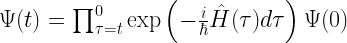
$\Psi (t) =\prod_{\tau=t}^{0}\exp\left(-\frac{i}{\hbar}\hat{H}({\tau)d\tau}\right)\Psi (0)$

with the product order going from left to right, however, if you so choose to do so, you can go the reverse route though it’s imperative to know that the reverse limits the multiplicative integration. Also, this does nothing in the matter of solving the problem.

For time-ordered continuous products, the notation goes like this

${\mathcal T}\exp\int_0^t H(t') \ (dt')$

${\mathcal T}$

…represents what’s called the time-ordering operation. Please note that the product integral was conceived by Volterra to aid in solving linear systems of differential equations. In regards to ordinary functions, product integrals come to play in the reduction of the ordinary integral which is probably why it lacks much mathematical clout–and of course, that depends on who you ask.

–Desmond (DTO™)

References and Sources

Title: Optimized Dynamical Decoupling for Time Dependent Hamiltonians

Date: October 2nd, 2009; March 16th, 2010

Authors: Stefano Pasini, Götz S. Uhrig

Abstract: The validity of optimized dynamical decoupling (DD) is extended to analytically time dependent Hamiltonians. As long as an expansion in time is possible the time dependence of the initial Hamiltonian does not affect the efficiency of optimized dynamical decoupling (UDD, Uhrig DD). This extension provides the analytic basis for (i) applying UDD to effective Hamiltonians in time dependent reference frames, for instance in the interaction picture of fast modes and for (ii) its application in hierarchical DD schemes with $\pi$ pulses about two perpendicular axes in spin space to suppress general decoherence, i.e., longitudinal relaxation and dephasing.

Title: On Schroedinger Equation with Time-Dependent Quadratic Hamiltonian…

Date: December 10th, 2009; December 11th, 2009; April 9th, 2010

Author: Erwin Suazo

Abstract: We study solutions to the Cauchy problem for the linear and nonlinear Schroedinger equation with a quadratic Hamiltonian depending on time. For the linear case the evolution operator can be expressed as an integral operator with the explicit formula for the kernel. As a consequence, conditions for local and global in time Strichartz estimates can be established. For the nonlinear case we show local well-posedness. As a particular case we obtain well-posedness for the damped harmonic nonlinear Schroedinger equation.

–Desmond (DTO™)

Share Arheliean™:

Related