According to the Gauss law, physical states must be charge-neutral. The Gauss law must not be interpreted as an operator equation seeing how it would directly violate the operator algebra / commutation relations. Therefore, it is translated into a constraint equation for the physical sector of the theory:

$G (x) = \nabla E (x) + \rho (x)$

$G (x) | \text {phys} \rangle = 0$

Now, you should be able to integrate the following equations:

$\int_V d^3x G (x) = \oint_{\partial V} dA E (x) + Q$

$[Q - \text{surface charge}] | \text{phys} \rangle = 0$

A universe with a closed topology is equivalent to a vanishing surface. Understandably, the boundary must be equal to zero, meaning for $S^3$ , $T^3$ and on, the total charge must be exactly zero. In regards to an open universe, you could introduce surface charges but it seems to be rather unnatural as these surface charges would then cancel the volume charges. As a result, it would mean that the Gauss law is equivalent to vanishing total charge.

In classical electromagnetism, we could say that the Gauss law is the directly mathematical result of imposing a twice differentiable vector field on a pseudo-Riemann manifold. Let’s say, A is a representation of the vector field. An expression of this would be J = -*d*dA, where J is the current and charge density all expressed in differential k-forms. The result is Gauss law combined with Ampere’s law (these two “laws” mirror each other), each expressing a part of this “law” in a different subspace of space and time. Seeing how J is the current and charge density and essentially a second derivative of A, which is the combined electric and magnetic potential. So, J is really nothing new, only a derivative of the vector field (A).

Charge is defined as the divergence of the electric field rather than a distinct [physical] quality that just so happens to be exactly equal to the divergence of $E$ . For a better explanation, we’ll have to look at QED (quantum electrodynamics) and QCD (quantum chromodynamics).

We have the physical gauge fields, which are two polarizations out of four A-components following gauge fixing; in QED it’s in the photons. In QCD, what are known as gluons have an additional color index. In addition to the physical gauge fields, you have be alert of the physical fermion spinor fields, $\psi$ , as well. As far as electromagnetism goes {for the matter of the electrons), in quantum chromodynamics, the quarks are now with an additional color index. In this case, the currents are neither defined in terms of a vector potential nor are they introduced as classical sources. Rather, they’re now defined via the fermionic degrees of freedom and, as a result, are independent physical objects.

$j^\mu = \bar{\psi} \gamma^\mu \psi$

The Gauss law relates the 0-component of the current [read: charge] living in the fermionic sector of the Hilbert space with the divergence of the E-field living in the bosonic (gauge field) sector of the Hilbert space. This is one of the reasons why they can’t be identical and that’s why the equation divergence electric field = fermionic charge density no longer hold as an operator equation; however, it remains valid as an equation acting on physical states which are defined as the states on which the Gauss law operator vanishes, i.e., eigenstates of the Gauss law with an eigenvalue of zero being equivalent to the kernel of the Gauss law. The Gauss law acts a generator of gauge transformations, A°=0 gauge with time-independent gauge transformations left. Therefore, vanishing of the Gauss law on physical states is equivalent to gauge invariance in the physical subspace. In contrast to electrodynamics, the Gauss law in quantum electrodynamics engages us about the relation between of the dynamics of the bosonic and the fermionic degrees of freedom.

The Gauss law does not say anything regarding the individual portions of the total charge; it only refers to the total charge in whole. This charge-neutrality condition would be conducive to the Gauss law:

$({N})_{proton} ({q})_{proton} + ({N})_{electron} ({q})_{proton} = 0$

^A little bit oversimplified, wouldn’t you say? You would have to use quarks in place of protons–not to mention all of the other charged particles.

For those of you pondering on the measurement of neutral-atoms, note that the measurements show that the total charge of one single atom vanishes; the Gauss law applies not to single atoms though there could be slightly charged atoms with a corresponding anti-charge located at the spatial infinity. However, these anti-charges would create electric fields that would show up in measurements.

In regards to the application of the Gauss law in addition to neutron radioactive decay in both a proton and an electron proving whether or not the magnitudes of electron and proton charges are exactly equal, you’ll need to know that if applied to a single neutron–one can see no mechanism in the matter of a neutral neutron delaying a charged electron-positron pair, plus neutral neutrinos. Not only that but you have to factor-in corresponding anti-charge located at spatial infinity. Mathematically, one could prepare a state |neutron> and describe its decay channel

|proton, electron, neutrino>

…which again, has vanishing total charge. As this process is localized there, in no way can it create an anti-charge at spatial infinity in order to cancel out total charge in the decay channel.

Come to think of it, the Gauss law is an exact equation of constraint which follows directly from the electromagnetic Lagrangian plus gauge condition A° = 0 (a good choice since A° isn’t a dynamical degree of freedom because of no canonical conjugate momentum).

Let me speak a little bit on the mechanics of the electromagnetic Lagrangian. Lagrangian mechanics is beautiful way to solve problems. You must know that the Lagrangian, $L$ , is written like $L=T-U$ with $T$ as a representation of the kinetic energy and $U$ representing the potential energy. Next, you’ll need to look for good choices of coordinates such as

x = r sin (theta) cos (phi)

y = r cos (theta) cos (phi)

z = r cos (theta)

Now, you’ll need to write the kinetic energy in spherical coordinates. As…

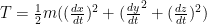
$T = \frac{1}{2}m( (\frac{dx}{dt})^{2}+(\frac{dy}{dt}^{2}+(\frac{dz} {dt})^{2})$

…you need to differentiate your three components with respect to time. The kinetic terms should turn out in trigonometric identities. Going back a bit, if you were to switch to a new coordinate system from the former, say…

ml2( θ2 + φ2 sin θ ) + mgl cos θ

The Lagrangian should look like this:

$\frac{m}{2} (r^2 + r^2{\theta}^2 + r^2 sin^2 {\theta}{\phi}^2) - rsin{\theta} cos {\phi}$

$r, \theta, \phi$ are variables that may have time dependence (if they didn’t the problem would be kinda dull since it would imply that the variables are constants in time and you would have a particle that wouldn’t move at all). The last part is knowing that it’s imperative that you understand the difference between partial derivatives and total derivatives. With partial derivatives, you have to derive the variable explicitly, meaning that the partial derivatives with respect to time of x would be 0, as there’s no explicit time dependence in the expression (i.e., no “t”). Total derivative implies you have to derive it all with respect to time, regardless if or not it is explicit.

In all honesty, Lagrangian dynamics can seem quite boring since you largely do not have to think all that much in regards to solving the problem. You just have to follow the order of steps.

Find a good coordinate system.
Know the general kinetic energy term in that system.
Place your constraints in the kinetic energy term if the system has any constraint.
Write your potential energy in these coordinates.
Write your Lagrangian.
Apply the Lagrange/Euler-Lagrange equations.
Have your motions of equations for the system.

In Hamiltonian mechanics, the total derivative with respect to time of the Hamiltonian is just the negative of the partial derivative with respect to time with the Lagrangian. Take the derivative of the Hamiltonian and plug in the definitions of the partial derivative and the Lagrangian equations of motion. The Hamiltonian is constant, provided the Lagrangian contains no explicit time dependence. This fact is possibly proved in your book somewhere but it is easy to get if you just use the equations of motion. Hamilton’s equations of motion are first-order differential equations while Lagrange’s equations of motion are second-order. Schematically, you’ll have

$\dot {q} = \frac{\partial H}{\partial p}$

and

$\dot {p} = - \frac{\partial H}{\partial q}$

If the Lagrangian is not explicitly time dependent, $\partial L/ \partial t = 0$ , then the Hamiltonian is now time independent, $dH/dt = 0$ .

Relating back to the topic of charged particles, I’ll need the quantization of all physical degrees of freedom would make the argument work, introducing classical/static charges without dynamics may spoil the argument when you consider the manipulation will permit the quantum dynamics to act on all charges the theory, on an immediate basis, will translate to you that the total charge must indeed vanish–provided that the manifold has no boundary.

In four-dimensional quantum field theory there are anomalies that are usually contained in so-called triangular graphs with three external gauge boson lines and three inner fermion lines forming a triangle with the graph being divergent and in need of being re-normalized. Typically, one would choose the method of renormalization such that the gauge current (the electromagnetic current) that’s derived from a local gauge symmetry remains conserved whereas the other current (axial current) is derived from a global symmetry becomes anomalous meaning the two currents are due to the fact that one can project to left-or-right-handed fermions, therefore, instead of calling in axial anomaly, one refers to it as a chiral anomaly. The reason being, that the gauge current conservation is renormalizability, or, the consistency of the proposed theory. The anomaly itself will have physical effects which can be seen in pion decay and the mass of the eta-prime meson. In electro-weak interactions, the left and right-handed currents evolve into gauge currents, conserved separately in classical field theory. However, due to aforementioned arguments, this involves that one can no longer protect both gauge symmetries in the current conservation because one must necessarily “break” gauge invariance in either the left or right-handed sector.

This means that the theory becomes inconsistent but there is one way to protect both gauge symmetries in the left–and the right-handed sector. Understand that each fermion species comes with its own triangle anomaly. However, the external gauge bosons do not carry any fermion information meaning that in order for one to calculate the total contribution of the triangle graphs to the current conservation you would have to come up with the sum over all triangle graphs. Know that each triangle comes with the pre-factor that is related to the [electro-weak] charges of the inner fermion within that same graph. With that in mind, the sum vanishes if the sum over these pre-factors vanishes which results in a constraint for the electro-weak charges of the fermions. So when speaking on the “standard model” (and how it factors into all of this), the anomaly has to cancel in each generation which essentially means that given the electric charge of the fermions and the multiplicity of the fermions in the graph (an example of this would be counting different colors), the electric charges must fulfill certain consistency conditions. Also, it means that one generation would indeed be complete. That’s one reason for the existence of the top quark; an incomplete third generation (e.g., bottom, tau, tau-neutrino) would cause the gauge current to become anomalous whereas a complete third generation (top, bottom, tau, tau-neutrino) would save the consistency.

Once you know that the electric charge of the electron, the charges of up and down are essentially fixed. The derivation would be both

Q(d) = – Q(u)/2

and

Q(d) = Q(e)/3

…the last equation is related to the fact that there are three colors–and the different colors are counted individually in the triangle diagrams. By using these equations you would automatically find that

$Q_({proton}) = 1 \text{and} Q_({neutron}) = 0 \text{in} \text{addition} \text{to} Q_({proton}) = - Q_({electron})$

There are processes in the “standard model” that violate certain symmetries that are somewhat considered classically valid via so-called anomalies, essentially nothing more than triangle diagrams [in Feynman diagrams, that is]. There are anomalies that are welcoming because they explain specific physical effects (pion decay, eta’ mass); these anomalies are usually due to global symmetries. Then, there are anomalies that must not exist as they would ruin the consistency of the “standard model”; these anomalies are due to local gauge symmetries. In quantum electrodynamics, there is no gauge anomaly as the left-and-right-handed fermions contribute with opposite sign and therefore the anomalies cancel, however, in the electro-weak interactions, the left-and-right-handed fermions couple differently to the gauge bosons meaning that the anomalies no longer cancel but that there are non-trivial conditions of consistency. You can consider it as a set of algebraic relations between particle-type specific parameters which are essentially the charges of these particles.

q(u) = 2/3 q(e)

q(d) = – 1/3 q(e)

Where you see 1/3, please note that is due to the fact that each quark is counted three times since it exists in three different colors due to this algebraic relation $q_({proton}) = - q_({electron})$ .

In reference to protons and neutrons–a proton consists of two quarks; one down quark and gluons that hold it together. A neutron consists of one up quark, two down quarks and gluons that hold it together. The decay process, in simple terms, occurs because a down quark changes into an up quark and emits an electron and an anti-neutrino. Note that the electron and anti-neutrino weren’t present before, they were created at the time this weak-force reaction took place.

It is correct to say: The neutron is composed of two up and down quarks.

Another thing to bear in mind is the fact that gluons will not couple to any particle that does not have color change so color-neutral particles will not couple to gluons, i.e., a gluon can affect a quark within a proton but it will not effect the entire proton and since the gluon is colored it’s not likely to bridge the gap between two orbiting protons in the manner that a pion would. Gluons that bind these quarks together would produce a cloud of quark-antiquark pairs everywhere they go, producing “seas” of quarks and anti-quarks in hadrons of all types [a quark-anti-quark pair is also known as a meson]. Mesons typically decay into other lighter mesons, or radiatively–via photon emission–especially in the case of system-heavy quarkonium–mesons won’t appear to have a strong tendency to decay into gluons though some may give off the appearance that they can. It is strictly dependent on the permitted paths of decay whether they are by quantum numbers, parity, charge-conjugation, etc. Since gluons are colored, they exist within an extremely strong field. Photons will couple into cascades of electron-positron pairs in an intense electromagnetic field or in a passing through barrier.

Quarks, on the other hand, are continuously emitting gluons and electrons can do this as well but with photons though.

References:

Phase Transitions, theta Behavior and Instantons in QCD and its Holographic Model

Authors: Andrei Parnachev, Ariel Zhitnitsky

Abstract: To elucidate the physics of the transition we consider a model where the chiral condensate does not vanish in the deconfining phase. The holographic model of QCD is a good example where this phenomenon occurs. On the field theoretic side this can be achieved by coupling fundamental matter to the hidden gauge group whose dynamically generated energy scale is higher than that of QCD.

Maximum Wavelength of Confined Quarks and Gluons and Properties of Quantum Chromodynamics

Authors: Stanley J. Brodsky, Robert Shrock

Neutron Beta Decay: Status and Future of the Asymmetry Measurement

Author: Takeyasu M. Ito

A clean, bright and versatile source of neutron decay products

Authors: D. Dubbers, H. Abele, S. Baessler, B. Maerkisch, M. Schumann, T. Soldner, O. Zimmer

Abstract: Chemical equilibrium among these particles is established by weak interactions such as neutron beta decay (n → p + e-+ ¯ v) and electron capture (e- + p→ n + v), and the nuclear symmetry energy plays an important role in determining the relative abundance of neutrons and protons.

Comparison of two experiments of radiative neutron decay

Authors: R.U. Khafizov, S.V. Tolokonnikov, V.A. Solovei, M.R. Kolhidashvili

Abstract: First, the results from the first experiment aiming to observe the as yet undiscovered radiative decay mode of the free neutron are reported. Although the experiment could not be performed under ideal conditions, the data collected still allowed one to deduce the B.R. = (3.2±1.6) 10 – 3 (99.7% C.L.) for the branching ratio of radiative neutron decay in the gamma region greater than 35 keV. This value is in agreement with the theoretical prediction based on the standard model, but because of the presence of a significant error (50%) we cannot make any definite conclusions. Taking into account the fact that the experimental conditions can still be significantly optimized, an e-p coincidence count rate of 5-10 events per second is within reach. Together with the standard model prediction for the branching ratio of this decay mode, this would correspond to a triple e-p-y coincidence rate of several events per 100 seconds. This can easily be observed with the current experimental set-up, which is now being optimized with a view to performing such an experiment. The aim of that experiment will then not only be to establish the existence of radiative neutron beta decay, but also to study B.R. in more detail. This, in turn, would allow to discover the deviation from standard electroweak theory. According to our estimates, we will be able to make more definite conclusions about deviation from the standard electroweak theory at the precision level of less than 10%.

C H A R G E – P A R T I C L E – M E N A G E R I E

-Desmond (DTO™)

-Desmond (DTO™)

Share Arheliean™:

Like this:

Related